My mother always told me “Everyone is special in their own way.” What she didn’t tell me, is that every cell in a spreadsheet is special too.

In this video, I will teach you how to go to a specific cell or range of cells using their special traits. This is perfect for jumping to a specific spot without scrolling, and for making mass changes in an extremely targeted and smart way. Get excited.

Download FREE Hands-On Exercises

Full Video Transcript:

Has your boss ever asked you to change the formulas to gray font and the numbers to blue font?

Well, in this video, I’m going to teach you how to do this in a few seconds instead of a few hours.

This shortcut has 2 components. The first is going to a very specific spot on your sheet if you know exactly where you want to go.

For example, if I want to go to a very, very low point, a high row number, but I don’t want to have to scroll, I would just do CTRL + G, and I would “Go To” for example, A9999, and I can just hit ENTER and I go immediately to that spot without any scrolling whatsoever. So, that’s a really simple way to move really quickly in a very targeted way, but the real, real power of this is to use the “Go To” with the “Special” option, all right?

So, when you hit “Special”, you’re going to choose a very special kind of cell, and I recommend you go through each one of these in more detail, but for now, let’s just look at, for example, a constant, and we can choose Only Numbers, Only Text, Only Logical, Only Errors, for example. Let’s choose Only Text.

It will scan through this entire sheet, and it will highlight, even if they’re not next to each other, all the cells that match that criteria, which means in one move now, I can make them all bold, or all italic, or anything. So, this is a very powerful way to do massive edits without having to search for it.

One nuance here is that you can actually choose the whole selection that you want first, and then it will match that criteria only within it. So, I’ll hit the Special with the ALT + S now to jump right to it, and I’ll go ahead and choose the ALT plus the letter to actually correspond to the underline here.

So, I want a Constant, so it’s ALT + O, and I’m going to uncheck the other ones that I don’t want, so ALT + U, ALT + G, and ALT + E to leave only the text. Hit ENTER, and now only these cells are selected, because I started first with that selection. If you choose nothing, it’ll go and look for the whole sheet as one.

I’ve created a series of exercises for you to practice and reinforce these Excel shortcuts. So, for example, you’re going to go to this worksheet over here and move the X’s by CTRL + X on the PC, COMMAND + X on the Mac, and then go to this exact reference by hitting CTRL + G, and GO35. It will jump to that spot, and you’ll know you’re in the right place because I put a little arrow for you. And CTRL + V on the PC or COMMAND + V on the Mac, and then you can actually keep going back and doing that for all of these.

The next exercise is to go to Special Cells. This one’s more involved, but you can totally get the hang of this as soon as you start going. So, make this side over here on the left match the format on the right in this very specific way, and if you want little hints, the legend here explains how it all works. So, anything that’s a text, right? You’re going to select this whole area here, you’re going to do your CTRL + G, and then your ALT + S on the PC to choose only the text. You’re going to turn off anything that’s not relevant, and then you’re going to apply the italics and the bold, and notice how it makes it match. So, do that for all of these and make the two images match.

Don’t forget to visit excelshir.com, where you can download these exercises, along with other free resources, such as keyboard shortcut cheat sheets for both PC and Mac.

Thanks for watching, and I’ll see you next time, but let me leave you with this parting thought. If a picture is worth a thousand words, then sharing the Excel love is priceless.

Picture this: you have a lot of reformatting to do on your spreadsheet and there are pockets of different formatting sprinkled throughout. Finally there’s a shortcut to speed up that process!

In this video, I will teach you how to select multiple cells that aren’t next to each other without touching the mouse.

Download FREE Hands-On Exercises

Full Video Transcript:

Have you ever tried to select multiple cells that were not next to each other?

Sure, there’s CTRL + CLICK for the PC. There’s COMMAND + CLICK for the Mac. But in this video, I’m going to teach you the shortcut to select non-adjacent cells using only the keyboard.

If you want to select cells that are not next to each other using the mouse, the way to do it primarily is with the keyboard, pressing and holding the CTRL key and then clicking with the mouse. This is probably what you’ve done thus far. You can even click and drag and get a whole range going. That’s for the PC. For the Mac, it’s the same thing, except instead of CTRL, you’re using COMMAND, keeping it pressed, and then clicking around that way.

However, if you ever want to use the keyboard only, the way to do it is with SHIFT + F8. And the memory trick is, “You should have come along, you funny mate!” Which is terrible, I know. This is a terrible trick, but hey, it actually helps you remember. The should is the Shift, and the “funny mate” sounds like eight, so it’s kind of like, you know, close, I guess.

Either way, the way to do it here is to keep SHIFT + F8 pressed now, and then move with the ARROWS. And what that does is it keeps that selection in place before moving. If I Shift down and to the right, for example, and then hit SHIFT + F8 again, I can safely move without losing that selection.

So that’s the whole trick. Before you move, you want to hit the SHIFT + F8. Otherwise, you will “lose your work,” right? If I hit SHIFT + ARROWS and then I move aside without hitting SHIFT + F8, I start from scratch. So that’s a big tip right there, is not to do that until you’re done and you actually have it all selected that you want.

So there’s one more nuance, which is that if you want to take an entire range, you’ll go ahead and hit SHIFT + F8 once, move aside, as we saw. But if you want to take a single cell, you’ll hit SHIFT + F8 twice before moving on. Otherwise, it will not work. So if it’s a single cell, you hit it twice. And if it’s a range of cells, you hit SHIFT + F8 once before you move.

I’ve created a series of exercises for you to practice this shortcut specifically. So the way to do it is to go to the “Non-Adjacent Ranges” tab. You want to match the format. Everything that’s on the left here, you want to make it look identical to the way it is in the example on the right. The only difference here is the bolding. But use the shortcut that we just learned.

So select all of these, hit SHIFT + F8, and then that way, you’ll get it all selected before you even apply the bold. And you would do it all in one swoop, and that’s kind of the whole benefit of this shortcut. That’s for the ranges.

The next tab is going to be the same thing but with individual cells. Notice, you’re going to hit SHIFT + F8 the first time just once, but afterwards, SHIFT + F8 twice before you move on. Otherwise, it will not work. And that’s the whole trick there.

Finally, if you’re feeling adventurous, you’ll go to this “Non-Adjacent Challenge” and you’ll do all of these in one selection without using the mouse. And that way, you can practice all of this together.

Don’t forget to visit excelshir.com, where you can download these exercises, along with other free resources, such as keyboard shortcut cheat sheets for both PC and Mac.

Thanks for watching. See you next time. And if you can only take a stand for one thing in your life, take a stand for sharing the Excel love. That sounds like someone I would stand for.

Wouldn’t it be nice if you could do a Google search on your spreadsheet?

Well, you can! And in this video I’ll show you how!

Download FREE Hands-On Exercises

Full Video Transcript:

Has it ever happened to you that you knew a specific phrase or even a specific number but you couldn’t seem to locate it on your spreadsheet?

Stop fumbling around and use this shortcut I’m about to teach you. It’s kind of like having a Google search on your spreadsheet.

You may think you know how to use Find but what I want to show you today is a way to really take advantage of this built-in feature, to locate exactly what you’re looking for without having to fumble around and just struggle.

So what you want to know is how to get to that Find box. That Find pop-up is CTRL + F, you may have already done this before. If I’m looking for an “X” and I hit ENTER right now, it’s going to go to the find next but if I keep going I can actually go to all the instances of it that way. Fundamentally, this is what it’s all about but there’s a lot of different ways to take it to the next level, which I’m about to show you.

So for example, if I go to the options, there’s a whole world of more advanced ways to go about this. You can do things like search for a specific format, we’re not gonna get into the details of it but I recommend that you explore this on your own time.

The cool thing is to search not just within the workbook, or not just within the worksheet, but the entire workbook, so for here, if I keep it within the sheet, it’s going to localize it to this worksheet only. You can search by rows, meaning going left to right and then down, like a book, or you can do it by columns, where it goes first up and down and then to the next column. Very cool way to speed up the search, if you have a lot of stuff.

You can also look within the formulas, within the value, within the comments, again, explore this on your own, match the case. I mean it’s crazy.

Really cool thing to do also, is to do a Find All, what that does is it gives you a list of all the different instances that that character or that string of characters appears. And you can see them all here, if I were to change it now to, say, within the entire workbook and I do Find All again, notice what happens, it gives me all the details. The cover worksheet has an “X” in it, in this cell, like, it literally lists everything out.

So I recommend that you explore this on your own, in detail. You can also go to the replace, and find every time there is an “X” and replace it with a “Y”, stuff like that, so it’s really, really cool.

To navigate this window, this is where it gets also pretty juicy, is to hit the TAB key and you’re going to jump to the next section of this pop-up itself. So TAB will go next, SHIFT + TAB will go to the previous, and if you’re on a checkbox, you want to hit the SPACE to activate or turn off the checkbox itself. ESC will essentially close the window without doing anything, and ENTER will actually save it or make that action take effect, and that’s what you want to keep in mind in terms of navigating this pop-up window.

Now, if you’re on a Mac, it’s a little bit different, I want to show you how this works. Anyone on a Mac can use the COMMAND + F but what that does is it gives you this little search box, and it’s not nearly as powerful as we just saw.

So instead, don’t hit COMMAND + F, resist the temptation, just hit CTRL + F and this is what you get instead, the same kind of options, not as much detail, but you still have more control than you did before. So that’s the nuance for Mac users, do not use COMMAND + F like you’d think to, use CTRL + F and you’ll get this more advantageous view.

I’ve created some exercises to help you reinforce all of these concepts that we learned, all these shortcuts. So again, what you want to do is go to that worksheet and find, here’s the hint, find the numbers. So I want to move the Xs, I’ll go ahead and do CTRL + X on the PC or COMMAND + X on the Mac and now, I’m going to find, CTRL + F, and look for the number one on this sheet only. And hit the next one, first it’s here, next it goes here, there’s one in there but that’s not what I wanted and now it goes to the one, which is somewhere on the sheet. We don’t know where, that’s why we’re using the find option here.

So go ahead and then you found it, close this up, go to the cell and CTRL + V on the PC or COMMAND + V on the Mac to paste, and go ahead and do that for all of the Xs for this exercise.

Don’t forget to visit excelshir.com, where you can download these exercises, along with other free resources such as keyboard shortcut cheat sheets for both PC and Mac.

Thanks for watching, and I’ll see you next time. And I’ve said it before I’ll say it again, share the Excel love.

This is hands down my favorite Excel shortcut, because I use it more times per day than I breath. Ok, I’m exaggerating, but not by that much.

This is a GAME CHANGER for anyone who spends any kind of time with spreadsheets. Without it, I wouldn’t just be slower, I’d be in tears.

In this video, I will show you the fastest way to move around a spreadsheet. Buckle up!

Download FREE Hands-On Exercises

Full Video Transcript:

This is one of the most important shortcuts you will ever learn because without it, you’ll be wasting countless hours, days, even weeks of your life.

In this video, I’m going to teach you the fastest way to move around a spreadsheet.

The way this works is, there’s a couple pieces to it. So, let’s start with an empty sheet, right? If I want to move it to the different cells with the keyboard, I’ll hit the ARROWS. That part’s pretty straightforward.

If I want to select as I go, go, I’ll hit the SHIFT key and then the ARROWS. Now, notice if I go to the right, it expands that way. If I go down, it expands down and I get this little rectangle. Then I go left. Notice how it’s kind of keeping that initial point as the selection start, but it will expand based on how I’m moving with the arrows as well.

So, think of SHIFT as “schlepping.” You’re taking it with you. You’re taking the selection with you as you go, hence schlep. Also sounds a little similar with the first letters, so that’s the idea.

The other piece to this is, if you want to move around really quickly, you can actually use the CTRL + ARROWS. So, notice where I am right now. I’m right over here. If I hit CTRL + LEFT, I will jump or “catapult” to the edge of the data. If I go CTRL + RIGHT, I’m going to catapult to the other edge, right? It’ll go down, left, up, it’s all going on these corners because that’s where the data is.

How, exactly, it works with the edge of the data is not super critical. You’ll get a feel for it as you go through. But basically, anything that has data in it, if it’s text, if it’s a formula, if it’s numbers, it’s all good as long as it’s not empty.

So, CTRL + ARROWS will catapult you to the next edge of the data. The really, really, really amazing part is to combine both things together. So, I’ll start over here. I’ll hit CTRL + SHIFT and then DOWN. I’ll select, as I go, that whole area. And I can expand the selection by doing CTRL + SHIFT to the RIGHT, and notice I got this whole section. So, this is where the real power comes in. You can combine the catapulting and the schlepping together. The CTRL + SHIFT + ARROWS.

Some Shir words of wisdom. What makes this so powerful is that you can actually use this concept when you are writing a formula as well. If I were to do, let’s say, a sum, I can actually do CTRL + SHIFT + DOWN and it’s going to keep that reference for me here, in the selection of those cells, inside of the formula. We’ll get to that a little bit later, but it’s one of those things that applies everywhere. I’m just going to undo that.

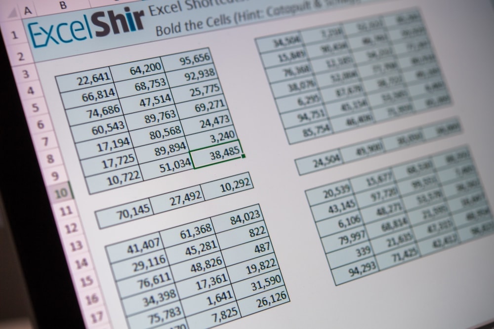
I’ve created some exercises for you to practice how to do this. So, if you’re going to start with the empty sheet, you can practice it by using the CTRL and the ARROWS to jump around. If you want to go to this worksheet over here, again, the point is to bold all of the cells and, of course to use the “catapulting” and “schlepping” as you go. So, a lot of these are a little different, but go through them and use the “catapulting,” the “schlepping” and bolding as you go.

Don’t forget to visit excelshir.com, where you can download these exercises along with other free resources, such as keyboard shortcut cheat sheets for both PC and Mac.

Thanks for watching. See you next time. And one quick story. I was watching a documentary the other day, and it turns out The Beatles broke up because they weren’t sharing the Excel love. Teachable moment.