Month: August 2017

0024 Excel Shortcuts: How to Change Font, Font Size, and Font Color (PC Only)

When it comes to Font Type, Font Size, and Font Color, you only really notice it when it’s bad.

Fortunately, once you know these Excel Shortcuts your spreadsheets will always stay clean and consistent.

(Only valid for PC, sorry Mac users)

Download FREE Hands-On Exercises

Full Video Transcript:

I’ve gotten countless spreadsheets where the font type, the font size, the font color were inconsistent and all over the place, and I know it’s because the person who made it didn’t know how to fix it quickly. In this video, I’m going to teach you how.

When you’re talking font type, font size and font color, it’s one of those things that you only really notice it when it’s bad. So, the way to make it look good is to use these shortcuts to actually get the result that you want and make everything clean and consistent.

With a PC, the trick to all of this is to hit the ALT + H + F, so Home, Font. And then it’s either going to be F for Font, S for Font Size, or C for Font Color. All right. So, let me start that process again.

I’m going to choose, first, the cell or cells that I want. Let’s choose this one. ALT + H + F + F. Right now, it’s Calibri. That’s pretty much the default. Let’s go a little wild. Let’s go Arial, right? And now it changes the font type completely.

Or I can change the font size with ALT + H + F + S, and make this a size 14 and it’s even bigger. I can also do ALT + H + F + C and choose the color that I want this way, as well. So that is how to get that moving.

Unfortunately, there is no option to customize your keyboard shortcut on the Mac. And so, really, what you have to do is use the Home tab on the ribbon, and go ahead and change the font type here, the font size and the font color with the little A symbol, because that’s referring to a letter on the screen. Pretty groundbreaking, I know.

Some final Shir words of wisdom for you is to actually think about it this way. Right. If you have a bunch of cells that contain formulas that are actually giving you an answer, that are calculated, I recommend that you use black font. And if you’re using an input where the user has to put something in themselves, use a blue font.

I didn’t make this up. This is a convention that exists for years and years. I think it’s awesome and it makes it a lot clearer where you input the cells that are blue and you don’t touch the cells that are black.

Speaking of not touching cells, let’s touch all of these cells in the next series of exercises. You want to go through and actually match the format on the left with the format on the right.

I’ve even given you some hints on what font types to use. It’s amazing. Go through each of these and change the font type. For example, over here, ALT + H + F + F, and Arial it and enter. You don’t get that fancy drop-down if you do it that way, but it’s okay because you don’t need to see it. You’re just actually going to be doing it yourself. It’s great.

You’re going to go to Font Size, change the font size on these to match the size indicated at the bottom. Font Color, if you can even read this. I can’t. I might need new glasses. That’s fine, too. And finally, if you’re feeling really adventurous, play a game of Pac-Man, and then fill out the font challenge here to make it look exactly the correct way with the font, font size and font color all wrapped into one. And then celebrate with a little champagne.

Don’t forget to visit excelshir.com where you can download these exercises, along with other free resources such as keyboard shortcut cheat sheets for both PC and Mac.

Thanks for watching. See you next time. And share the Excel love. It’s the gift that keeps on giving.

0023 Excel Shortcuts: How to Highlight Cells (Change Background Color) (PC Only)

Most people either highlight their spreadsheets way too much, or far too little.

But today, you’re going to learn the fastest and most effective PC Excel Shortcut to draw attention to specific areas of your spreadsheet.

(Valid on PC only. Sorry MAC users)

Download FREE Hands-On Exercises

Full Video Transcript:

This shortcut is the quickest, most effective way to draw someone’s attention to a cell or a range of cells. And now, you can finally do it with the keyboard if you’re on a PC. Sorry, Mac users.

Highlighting cells is important not just to make your spreadsheet look pretty, but to show your data in a clean, professional, and clear way that gets your message across.

I can’t even begin to tell you how many spreadsheets I’ve received that were complete eyesores. In fact, I can’t remember the last clean-looking spreadsheet I ever got.

So, if you think about it, if you’re highlighting everything, then all of a sudden, nothing stands out, so don’t be that person. Be very clean with your highlighting cells, and today, I’m going to show you not only how to do it, but how to do it efficiently and quickly.

On the PC, you’re going to have a whole bunch of ways to access the highlighting, all starting with the ALT + H, right? ALT is going to get us to the top here. ALT + H for Home, and then we’re going to go to H for Highlight Cells, and then we have a bunch of choices. So, we can actually go ahead and use the UP and DOWN arrows to choose the color we want and hit ENTER once we find that choice that we like.

It’s a little bit more manual, but there’s no other way to jump to the color you want specifically, unless of course, you’re doing something like ALT + H + H + N. Notice the N over here for No Fill, which actually removes it. In this case, a white background, which is not the same as everything else, so I don’t want that either.

The last choice is ALT + H + H + M for More colors, which brings us to this little popup where we have a whole bunch of choices and we can get very, very specific with the color scale, or we can choose from a list of standard colors, or actually get very exact, so that’s a nice way to do it.

Unfortunately, on the Mac, there are no keyboard shortcuts and you can’t even customize it, but what you can do is use the top Home ribbon and click on the Highlight Cells and do it the way that you’ve probably been doing it until now, because that’s the only option.

There’s not a whole lot to remember, because everything corresponds, so you’re going to highlight the cells, and then you’re going to go ahead and do No Fill, and M for More colors, so it’s all very straightforward.

There’s a bunch of other bonus shortcuts that all have to do with ALT + H + H + M, all to do with this screen here when you choose More colors. So, CTRL + PGDN will actually go to the next tab or CTRL + PGUP to go to the previous tab, things like that.

If you hit TAB, it’ll actually move to the next section. You can use the arrows and hit ENTER. It gets very fancy. You don’t have to worry too much about it, but it actually navigates within this window, and this is true, also, for many other popups that come up on your computer, so it’s kind of cool.

I’m going to hit ESC to get out of this, but what we cannot escape from is reinforcing these concepts, and we’re going to do that with exercises I’ve created for just this purpose. You’re welcome.

We’re going to go to this tab over here, and we’re going to see how we highlight the cells we want in the colors that we want. So, choose the cells here and go to your ALT + H + H and find that blue, whatever corresponding color we’re going for here. I believe it’s this one. I’m little colorblind, so I don’t know. I think that looks good, right?

The point is to make the left section over here look identical to the example on the right, so go ahead and follow those to the end, to fruition. You’ll notice here if you do No Fill, you might see some lines from borders. That’s because that’s the gridline that’s been there all along in the background, but in fact, when we’re using colors on these cells, it looks like we don’t have them anymore. So, if you see them again, that’s not a bad sign. That actually means that it’s working correctly. Don’t freak out.

The last one here is to choose exact colors using the More colors, and in fact, there’s a red, green, blue color scheme here for all of it. I’m sure you’ll do great. Have fun with that.

Don’t forget to visit excelshir.com where you can download these exercises, along with other free resources such as keyboard shortcut cheat sheets for both PC and Mac.

Thanks for watching, see you next time, and as a diehard Star Wars fan, I would be remiss if I didn’t leave you with this parting thought. May the force be with you as you’re sharing the Excel love.

0022 Excel Shortcuts: How to Copy and Paste Column Widths

After painstakingly changing your column widths, there’s no need to do that work over again. Just use the shortcut I’m about to teach you to copy and paste the column width in a snap!

Download FREE Hands-On Exercises

Full Video Transcript:

If you’re anything like me, you probably spent the better half of your adult life not knowing that you could copy and paste column widths in Excel.

Now that you know it’s possible, today I’m going to teach you exactly how to do it.

In the previous video, I showed you how to change column widths and row heights. You can actually go ahead and click on the link in the description in case you missed it.

Now that you’ve done that work already, I’m going to teach you how to copy and paste only the widths of the columns from one section to another, using a little something I like to call “Paste Special.” Since Microsoft calls it Paste Special too, that’s what we’ll all be calling it from here on out.

Paste Special’s one of those amazing things that, if you’re using it correctly, you’re saving yourself tons of time every single time that you’re using Excel, but if you don’t use it, you’re really missing out.

The key to it is to first choose and select the cell that has the quality that you want to it. For example, if I want to take this cell right here, and actually this entire column really, I’ll go ahead and expand the selection using CTRL + SPACE. I’ll do a little CTRL + C to copy it.

Now, I’m not going to paste the actual contents, but what I will do is paste the width of the column. I can go ahead and do CTRL + SPACE again to select this column here, or I can just choose a single cell and do CTRL + ALT + V. Now notice what happens. I threw an ALT in there. Instead of doing a regular paste with a CTRL + V, I’m using CTRL + ALT + V, which brings me to Paste Special.

And of course, the magic here completely is the column width. I can jump to this even quicker by using the ALT + W on the PC to get to that spot immediately. I’ll hit OK, and it’s now going to obviously give me an error message, because why not? In fact, that thing I said before, let’s make it width, and then it’s going to work. See, it’s always better to make it like to like. If you’re doing a whole column, then paste a whole column. Otherwise it’ll yell at you, basically.

That’s how you want to do it. I can hit ESC to get rid of these little borders here. It’s just showing it’s on the clipboard. The whole point is, you’re doing a Copy and a Paste Special with just the column width.

Let’s see this in the Mac. It’s very much the same thing. The whole point on the Mac is that instead of doing it with…let’s do, for example, over here. Same concept. I’ll do CTRL + SPACE to get the whole column, COMMAND + C to copy. I’ll do CTRL + SPACE to get this new column over here, and do CTRL + COMMAND + V to bring my Paste Special window up here.

The only difference is, I’m not going to do ALT, I’m going to do a fn + W. I hit the fn + W, it will get you to this spot right here. Then you do OK, and it will apply that width to there as well. Hit ESC to get rid of that.

If you want to lock in this shortcut, then let’s go ahead and go to this exercise, where you’re actually going to take the original column width over here, you’re going to copy it, and you’re going to paste it over to these.

It’s really, really simple, but the whole point is to get it to look like it does on the right. Use that shortcut and then do it as many times as you need to until you can do it with your eyes closed. Enjoy.

Don’t forget to visit excelshir.com where you can download these exercises, along with other free resources such as keyboard shortcut cheat sheets for both PC and Mac.

Thanks for watching. See you next time, and remember, every journey begins with a first step. May I suggest that first step be to share the Excel love. I read it in a fortune cookie once. It was delicious.

0021 Excel Shortcuts: How to Change Column Width and Row Height

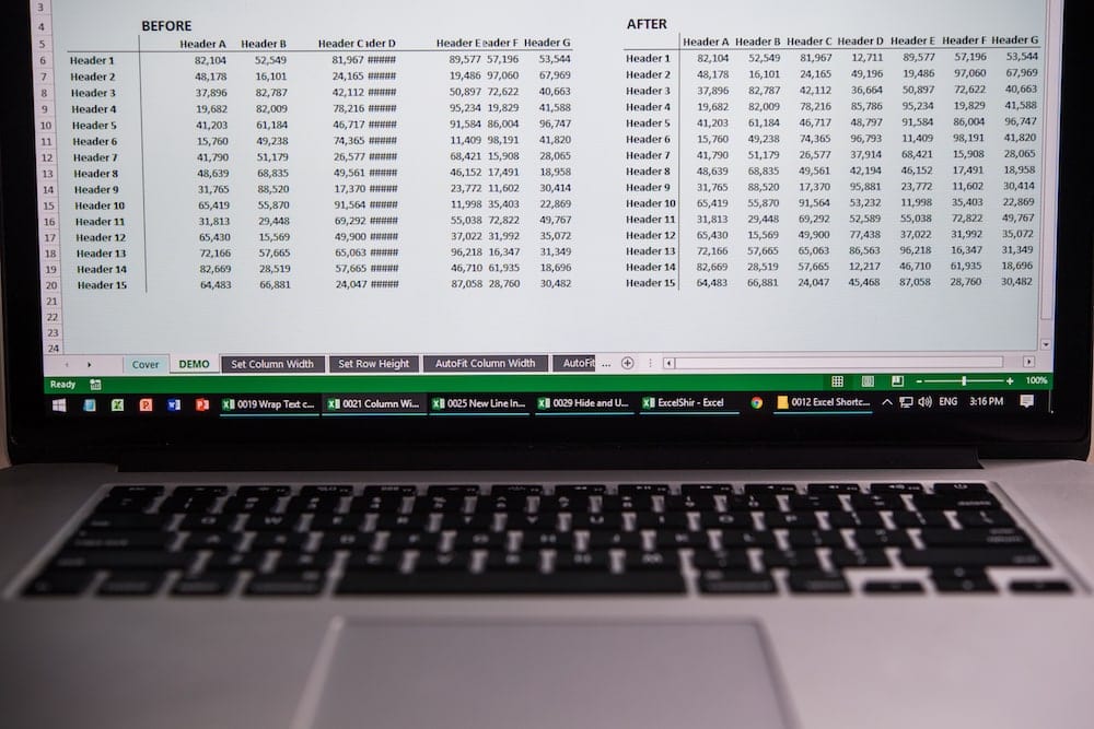
You know those annoying # signs that pop up on your spreadsheet every once in a while? It’s because your columns aren’t wide enough!

In today’s video, I’m going to teach you how to change the column width and row height with laser-like precision and speed.

Download FREE Hands-On Exercises

Full Video Transcript:

If you’re still using the mouse to adjust the column widths manually, I guarantee you that you’re leaving minutes on the table every single day.

Minutes that you could be spending getting coffee, gossiping with coworkers, or watching videos of corny Excel instructors.

No matter what industry you’re in or what your job is, or pretty much what you’re doing with your life, you will always need to change column widths and row heights. It’s just a fact of life. It’s just how it is.

There’s two main approaches. You can do the quick and dirty approach, and the precise guess and check. Quick and dirty refers to AutoFit, and the guess and check refers to changing the exact column width or row height. So, let me show you both.

If you’re on a PC, you want to go ahead and use the ALT + H + O + W to set the column width. Now, notice something about all of these is that they’re based on the current selection. So, for example, if I take all of this here and I want to expand it to fit all of them, I’m not just going to go ahead and click this way because that takes me forever.

Instead, I’m going to select all of these and do ALT + H + O, right? H for Home, O for Format, and I want to do a W for Width. If I wanted to guess exactly how much, because I’ve been doing this a long time, I’m going to guess probably, like, 14, and it’s pretty close, right?

But if I want it to be exact, I would do ALT + H + O + I to AutoFit, which is a really big time saver, and it’s based on the selection, meaning if I do ALT + H + O + I here, it’s going to fit only to this level. If I want to do the entire column, ALT + H + O + I.

If I, you know, hit ALT first, it’ll work, and it’ll give us to all of that because I have a lot of text underneath, so be aware of what you’re selecting before you actually put that shortcut into effect.

If you want to do the row, in contrast, it’s going to be ALT + H + O + H for the Row Height. Usually the default is 15. Or you can actually go ahead and do ALT + H + O + A to AutoFit the row height.

So, how do we remember all this? There’s a couple really corny Santa Claus tricks here, so just bear with me.

W is for width, which is super easy. H is for height, but for the I and the A, just think of the I as, like, suck it in, Santa, and the fact that I is, like, the most narrow vertical line anyway, so it will, you know, suck it in, basically.

A is, like, think of an attic, and you got to watch your head in the attic because they have low ceilings. You want to fit that row so it’s nice and snug, and it’s really compact. So, again, you always start with the H + O. That’s why I thought of Santa Claus. HO HO HO HO, get it? Okay.

And then there’s the Mac equivalent, which is all based on the customized shortcuts. So, go ahead and go to the description of this video and click on the link to go step-by-step on how to create your own Mac keyboard shortcuts. otherwise these will not work at all. So, again, I chose similar keys so that it’s actually very much related to the same as the PC.

Wishing you had your own exercises to follow along with? Well, fortunately, they’re right here. Just go ahead and actually follow through with each of these to the point where the left side looks exactly like the right. And you’ll notice that the numbers themselves are different on the PC than on the Mac, but again, just use the ones that correspond to the system that you’re using.

So, If I have a PC here, I’m going to keep the default at 8.43, but this one I’m going to do ALT + H + O + W and get the 9 here and hit ENTER, and it’s going to adjust it for me that way.

So, I’m going to go through each one. You can select a single cell or the entire column if you’re doing the Adjust Width with ALT + H + O + W because it’ll affect the whole column anyway. So, that’s for the Set Column Width.

Similar thing with the row height, and then you’re going to do AutoFit. So, be aware of what you’re selecting first. That’s the trick to this whole thing to make it look exactly like this. You’ll get a feel for it and see how it works, but, basically, that’s it, and then when you’re done, you want to actually go ahead and make sure that everything wraps up nicely.

The trick to this whole thing is that when you’re using Wrap Text, things can get a little bit weird because it doesn’t know how you want to, basically, AutoFit them. So, what I mean by that is…I’m going to do a little AutoFit of the row. So, ALT + H + O + A is how I get this point, but I don’t know. If I do ALT + H + O + I it’s going to cut it off here, but if I’m over here, for example, and I do ALT + H + O + I, it’s different.

It doesn’t always know what to do, so this is more of the art of Excel than the science. So, kind of get it most of the way there first, but then get more precise by doing ALT + H + O + W and maybe doing it to a four. And then you can snug it in so it’s already cut off at the right word, that kind of thing. So, again, just play with it and get the feel for it, but basically, have fun and learn.

Don’t forget to visit excelshir.com where you can download these exercises, along with other free resources such as keyboard shortcut cheat sheets for both PC and Mac.

Thanks for watching, see you next time, and one last exercise. Think of the person you love the most. Call them up and share the Excel love. Sharing is caring.