Tag: Tutorial

0021 Excel Shortcuts: How to Change Column Width and Row Height

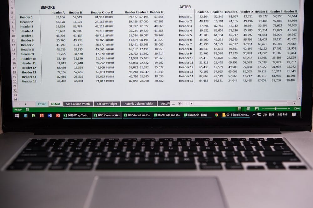
You know those annoying # signs that pop up on your spreadsheet every once in a while? It’s because your columns aren’t wide enough!

In today’s video, I’m going to teach you how to change the column width and row height with laser-like precision and speed.

Download FREE Hands-On Exercises

Full Video Transcript:

If you’re still using the mouse to adjust the column widths manually, I guarantee you that you’re leaving minutes on the table every single day.

Minutes that you could be spending getting coffee, gossiping with coworkers, or watching videos of corny Excel instructors.

No matter what industry you’re in or what your job is, or pretty much what you’re doing with your life, you will always need to change column widths and row heights. It’s just a fact of life. It’s just how it is.

There’s two main approaches. You can do the quick and dirty approach, and the precise guess and check. Quick and dirty refers to AutoFit, and the guess and check refers to changing the exact column width or row height. So, let me show you both.

If you’re on a PC, you want to go ahead and use the ALT + H + O + W to set the column width. Now, notice something about all of these is that they’re based on the current selection. So, for example, if I take all of this here and I want to expand it to fit all of them, I’m not just going to go ahead and click this way because that takes me forever.

Instead, I’m going to select all of these and do ALT + H + O, right? H for Home, O for Format, and I want to do a W for Width. If I wanted to guess exactly how much, because I’ve been doing this a long time, I’m going to guess probably, like, 14, and it’s pretty close, right?

But if I want it to be exact, I would do ALT + H + O + I to AutoFit, which is a really big time saver, and it’s based on the selection, meaning if I do ALT + H + O + I here, it’s going to fit only to this level. If I want to do the entire column, ALT + H + O + I.

If I, you know, hit ALT first, it’ll work, and it’ll give us to all of that because I have a lot of text underneath, so be aware of what you’re selecting before you actually put that shortcut into effect.

If you want to do the row, in contrast, it’s going to be ALT + H + O + H for the Row Height. Usually the default is 15. Or you can actually go ahead and do ALT + H + O + A to AutoFit the row height.

So, how do we remember all this? There’s a couple really corny Santa Claus tricks here, so just bear with me.

W is for width, which is super easy. H is for height, but for the I and the A, just think of the I as, like, suck it in, Santa, and the fact that I is, like, the most narrow vertical line anyway, so it will, you know, suck it in, basically.

A is, like, think of an attic, and you got to watch your head in the attic because they have low ceilings. You want to fit that row so it’s nice and snug, and it’s really compact. So, again, you always start with the H + O. That’s why I thought of Santa Claus. HO HO HO HO, get it? Okay.

And then there’s the Mac equivalent, which is all based on the customized shortcuts. So, go ahead and go to the description of this video and click on the link to go step-by-step on how to create your own Mac keyboard shortcuts. otherwise these will not work at all. So, again, I chose similar keys so that it’s actually very much related to the same as the PC.

Wishing you had your own exercises to follow along with? Well, fortunately, they’re right here. Just go ahead and actually follow through with each of these to the point where the left side looks exactly like the right. And you’ll notice that the numbers themselves are different on the PC than on the Mac, but again, just use the ones that correspond to the system that you’re using.

So, If I have a PC here, I’m going to keep the default at 8.43, but this one I’m going to do ALT + H + O + W and get the 9 here and hit ENTER, and it’s going to adjust it for me that way.

So, I’m going to go through each one. You can select a single cell or the entire column if you’re doing the Adjust Width with ALT + H + O + W because it’ll affect the whole column anyway. So, that’s for the Set Column Width.

Similar thing with the row height, and then you’re going to do AutoFit. So, be aware of what you’re selecting first. That’s the trick to this whole thing to make it look exactly like this. You’ll get a feel for it and see how it works, but, basically, that’s it, and then when you’re done, you want to actually go ahead and make sure that everything wraps up nicely.

The trick to this whole thing is that when you’re using Wrap Text, things can get a little bit weird because it doesn’t know how you want to, basically, AutoFit them. So, what I mean by that is…I’m going to do a little AutoFit of the row. So, ALT + H + O + A is how I get this point, but I don’t know. If I do ALT + H + O + I it’s going to cut it off here, but if I’m over here, for example, and I do ALT + H + O + I, it’s different.

It doesn’t always know what to do, so this is more of the art of Excel than the science. So, kind of get it most of the way there first, but then get more precise by doing ALT + H + O + W and maybe doing it to a four. And then you can snug it in so it’s already cut off at the right word, that kind of thing. So, again, just play with it and get the feel for it, but basically, have fun and learn.

Don’t forget to visit excelshir.com where you can download these exercises, along with other free resources such as keyboard shortcut cheat sheets for both PC and Mac.

Thanks for watching, see you next time, and one last exercise. Think of the person you love the most. Call them up and share the Excel love. Sharing is caring.

0020 Excel Shortcuts: How to Add and Remove Borders

FACT: Most Excel files either have way too many borders, or not enough. The reason? Formatting borders with the mouse is inconvenient and time consuming.

The solution? Watch this video and learn 6 Excel shortcuts for the most common border formats.

Download FREE Hands-On Exercises

Full Video Transcript:

Can I ask you a personal question? How much time are you spending creating borders? If it’s any more than a few seconds, you’re taking way too long.

But don’t worry, in this video, I’ll show you how to create the exact borders you want, fast.

We all know borders are important because it separates information, like headers or total rows from the rest of the table.

But the real question is how do we create the exact borders we want and how do we do it efficiently? We can actually do it very, very fast and very efficiently with the following shortcut.

So for the PC, we want to do things like CTRL + SHIFT + & to create an outside border on the current selection. Let me show you how this works, right? If I’m over here and I do CTRL + SHIFT + &, it looks like nothing happened, but as soon as I move the selection away, I’ve left that outside border there in place. It’s there, it’s waiting, it’s awesome.

You can even select a few different cells and then do that shortcut CTRL + SHIFT + & and then you move aside and you get that same effect.

Let’s go to the next shortcut. Over here is the CTRL + SHIFT + _ (Underscore) to remove the outside border from the current selection. So, if I want to take this one only, I can do CTRL + SHIFT + _ (Underscore) and it’s going to remove it, or I can take an entire selection like this and overlap it that way, if I want to save some time to do it across the board.

The memory trick here is to think of it as an ampersand, you’re adding a lot of borders, hence the outside, everything up on a perimeter of the current selection.

The underscore is like a blank, so you want to fill in the blanks, right? It’s going to remove whatever border you had on the outside.

The next series of shortcuts are going to be a little bit more involved, in the sense that we have the ALT + H + B and then a letter. So, the way that works here is…let me show you each example. ALT + H + B Home Border and we get a ton of options, but we don’t want to use all these because they’re not as useful.

In fact, the P is really helpful because it’s going to be the top. Now, T was already taken, but P, you want to think of it as popping the top off the Pringles. It’s a lot of P’s in the sentence but it basically helps you remember to put it towards the top, right?

If you want to do the bottom, it’s ALT + H + B + O for the bottom. Think of O as like, the original flavor of Pringles, which is the bottom of the barrel, because some people hate it, apparently. And you can also think of it as like a Pringles can on a table and tracing a pencil around it and it draws a little O there. So ALT + H + B + O will get you to the bottom of whatever the current selection is.

In contrast, ALT + H + B + L is for left border, ALT + H + B + R is for right, those are really straightforward. So again, you can do all the directions you want based on the current selection if you just start with the ALT + H + B and then a letter that corresponds to the border that you want.

Things are a little bit different for the Mac. So, if we want to go back to the other sheet here, we’ll see that, in fact, the same things can be achieved, but it’s done a little bit differently.

So, with the Mac, you want to use the OPT + COMMAND + 0 (Zero) to add the outside border. If you look at it, it’s kind of like an outside perimeter. Sort of. But basically, helps you draw the outside border.

If you do the OPT + COMMAND + _ (Underscore), that’s the same to remove the outside border, and then this is one of those rare cases where Mac is better than a PC, in terms of the default shortcuts, because you just use the arrows. You do OPT + COMMAND + UP up to create a top border, DOWN for a bottom border etc. etc. I think that’s awesome and I love that about the Mac shortcuts there. So, if you have a Mac, enjoy it while you can.

Let’s see these bad boys in action, right? Go ahead and go to these different tabs and actually complete these exercises. So, you want to make the left section here match with the right section in the example, and use the borders shortcuts that we just learned.

So, select the cells you want first and then put into effect the actual shortcut CTRL + SHIFT + &, in this case, and you’ll just go through and fill in everything until it looks identical and until you pretty much have this down cold. So, go ahead and practice it for the outside border, removing borders, top, bottom, left, right, and if you’re feeling fancy, little challenge, anyone want to play pong, anyone? Yeah? Okay, great.

Don’t forget to visit excelshir.com where you can download these exercises, along with other free resources such as keyboard shortcut cheat sheets for both PC and Mac.

Thanks for watching and I’ll see you next time. And share that Excel love. Yeah, it’s contagious.

0019 Excel Shortcuts: How to Wrap Text (PC Only)

Have you ever had text get cut off because the cell wasn’t wide enough? Wrap Text is what’s been missing in your life, and your spreadsheet.

In this video, I will teach you how to maximize the space on your spreadsheet with one simple shortcut for PC (sorry Mac users).

Download FREE Hands-On Exercises

Full Video Transcript:

Have you ever widened a column so much just so that you could fit all the text, and have a whole bunch of white space left over? Stop immediately.

In this video, I’m going to teach you how to actually wrap text quickly and correctly.

This shortcut is really important because it lets you take full advantage of the space that you have on your spreadsheet, on your screen, and pretty much in your life, right?

I’ve had clients where they had columns that were way too wide and was just taking up all the space because they didn’t know how to wrap text correctly, and so we couldn’t even see all the relevant information on the screen at the same time. We had to scroll back and forth, it was a waste of time, it was frustrating. The whole point is to be concise, get everything nice and neat on your screen.

The way to do Wrap Text with a PC is to hit ALT + H + W. It’s going to give you the same spot here on the top ribbon, and the whole thing is, it’s a “sticky key.” When you hit ALT, it is a sticky key because you’re pressing and letting go and that means it’s still waiting for your next move.

You’re going to hit H for Home and W for Wrap Text. So again, you want to keep in mind what you’re selecting first before you do this, otherwise it’ll just wrap the wrong thing, essentially.

Sadly, for the Mac, there is no keyboard shortcut for this and you can’t customize it, but what you can do is go to the top ribbon on the Home tab and hit Wrap Text on the Mac and you’ll get the same result. Or you can get into the same Format Cells with command one and go to the Alignment tab and change the Wrap Text that way.

Let’s see this in action with an exercise that’ll help us remember and actually internalize this shortcut. So, go ahead and go to this Wrap Text tab and match the left side to the example on the right. So again, select first. Choose all the cells that you want to make have this change, and then do ALT + H + W and it’s going to wrap them so that you can see everything nicely versus having to do it the old-fashioned way and spend way too much time and space to do it that way.

Instead, you’re going to choose those cells and you’re going to ALT + H + W and make it look clean, nice and concise.

Don’t forget to visit excelshir.com where you can download these exercises, along with other free resources such as keyboard shortcut cheat sheets for both PC and Mac.

Thanks for watching and I’ll see you next time, and in the meantime, don’t forget to share the Excel love.

0018 Excel Shortcuts: How to Align Cells

Cell Alignment isn’t just for the obsessive excel user, since it can singlehandedly make or break the overall presentation of a report. I’ve sat in on year end evaluation meetings before, trust me.

In this video, I will show you how to align cells consistently every time with a few simple excel shortcuts.

Download FREE Hands-On Exercises

Full Video Transcript:

Nothing will drive a person crazier than when cells do not line up.

I kid you not. I had a client once whose entire purpose for hiring me was to line up the cells in a report.

And it might seem trivial, but in fact, this can make or break the professionalism of a report. And today I’m going to show you how to do it.

Whether you’re aware of it or not, you are already aligning cells left, right, center, all the time, but you’re probably using the mouse. And today I’m going to show you how to use the keyboard to cut that time down significantly.

It really comes down to a very straightforward series of steps. The whole beginning is to hit ALT + H for Home and A for Align, and then it’s going to be a letter that corresponds to the action itself, so L for Left, C for Center, R for Right. I mean it doesn’t get more straightforward than this. T for Top, M for Middle, B for Bottom. Just go straight with that, and you’ll be on a very good footing.

The whole point is to get to this top ribbon piece with the PC, and then you’re golden. There’s really not too much to remember. It’s all baked into it. If you’re on the Mac, on the other hand, the two that are built in are COMMAND + L for the Left and COMMAND + E for Center. And because C was already taken, you have to use E and think of it as Equidistant from both sides.

Unfortunately, on the Mac, you cannot customize the keyboard shortcuts for the rest of these, for the right, top, middle or bottom, so you’re going to have to use the ribbon on the Mac to actually do it the other way. But otherwise, you’re going to save a considerable amount of time by using these keyboard shortcuts to align your cells.

Let’s illustrate these shortcuts with a few specific exercises. So you’ll have the align left. Again, just make this left section here match the exact format on the right and use the keyboard shortcut to make it happen.

So once you’re here, ALT + H + A + L for the Align Left. And you’ll go through and you’ll actually practice it several times until you get it down cold. We have it for the left, for the center, for the right, top, middle and bottom. And of course, a nice little challenge to get it to match up exactly.

Don’t forget to visit excelshir.com where you can download these exercises, along with other free resources such as keyboard shortcut cheat sheets for both PC and Mac.

Thanks for watching. See you next time. And if there’s just one thing you do today, share the Excel love. It will make you feel all warm and fuzzy on the inside.

0017 Excel Shortcuts: How to Change Number Formats

I wouldn’t show this as a party trick at your next soirĂ©e, but I would use this when creating a quick back-of-the-napkin spreadsheet.

In this video, I will teach you how to quickly format your numbers 7 different ways without touching the mouse.

Download FREE Hands-On Exercises

Full Video Transcript:

Don’t you hate it when you’re typing out a list of numbers and some appear with a decimal, some with no decimal, some with a comma, some with a currency symbol, and all you wanted is to get them all to look the same?

This video is for you because I’m going to teach you exactly how to format your numbers quickly, efficiently, and correctly.

In the previous video, I showed you how to format your spreadsheet precisely and comprehensively. There’s actually a link in the description below, in case you missed it.

In contrast, this video shows you how to get the most common formats really quickly, for those back-of-the-napkin type calculations that you just need more quickly.

So here is a list of all of the quick formatting shortcuts. The trick to all of this is CTRL + SHIFT + Something, and that something is going to be on that entire, basically, half of that row on the keyboard on the top, starting with that Grave symbol, which you may not have used ever before, all the way through 1 through 6.

So if you do CTRL + SHIFT and one of those, you’ll get the format that corresponds to it. So CTRL + SHIFT + ` (Grave) will get you general. G, grave, general. Get it? It’s all related. Okay.

Exclamation point is because you’re going to do the number, right? Think of it as like the decimal point that appears when you do it. The @ is like, “What time is the party at?” So I want to see the time. That’s how that’s working.

The hashtag here, the little date thing, I always think of, you know, being stranded on a deserted island and counting down the days with little tick marks. So that makes me think of the day format.

Currency is straightforward because it’s a dollar sign. Percentage is a percentage. This one is a little caret, or caret, depending on how you want to pronounce it, and it’s going to be raising the scientific roof because basically it’s scientific notation. So the numbers are too big or too small, actually, and you need to show it in a scientific format.

That’s essentially it, and it’s the same exact shortcut for the Mac. It’s still CTRL + SHIFT, and then that other additional number or the Grave symbol on the left of the 1.

Pull up a chair because there’s a bunch of shortcuts to work through here, right? We’ve got the general. So you want to make the entire left section over here match the format on the right. And all you have to do is turn these cells into the correct format, CTRL + SHIFT + ` (Grave), and it will go ahead and match it to that spot.

Go through each of these using the shortcut that we talked about. There might be some subliminal messaging here, which is not so subliminal anymore because I talked about it, but you get the idea. Go through each of these, and then go through the challenge one where every single one of these should match in a very precise way. And really just practice as much as you need to until you get it memorized.

Don’t forget to visit excelshir.com where you can download these exercises, along with other free resources such as keyboard shortcut cheat sheets for both PC and Mac.

Thanks for watching. See you next time. And tonight, before putting your kids to sleep, instead of reading them a bedtime story, share the Excel love. Trust me. Knocks them right out.